This article aims to explain core intuition behind Stable Diffusion with detail.

Table of Contents

1. Introduction
   • Intuition of Probability Distribution
   • How This Applies in Image Generation
2. Data Representation
   • Raw Pixel Space
   • Better Data Representations
3. Variational Autoencoders (VAE)
   • Before VAE: Autoencoder (AE)
   • VAE Components
   • Loss of VAE
4. Diffusion Process
   • Noise and Denoising Intuition
   • Training (Forward & Backward Process)
   • Alternative Perspective (Latent Space View)
5. Inference
   • Generating Images from Noise
   • Interpolation in Latent Space
6. Conditioning
   • Intuition
   • Distribution View
7. Core Architecture
   • U-Net
   • Self Attention
   • Cross Attention
8. Wrap Up

Introduction

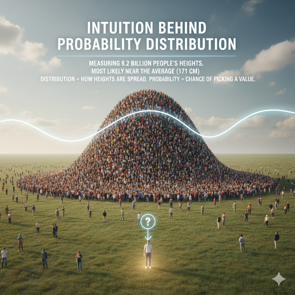
Intution behind Probability Distribution

Imagine measuring the height of Earth’s 8.2 billion people. If you randomly pick one person, you’ll most likely get a height near the average (about 171 cm). A distribution shows how all those heights are spread out. Probability tells you the chance of picking a particular value.

How This Applies in Image Generation

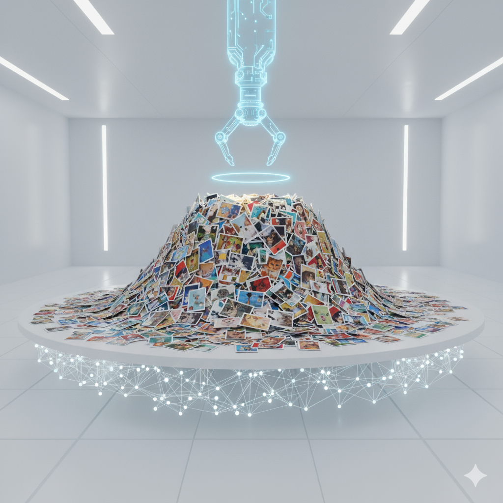
Now let’s align that idea to diffusion model. You can think of diffusion model as a machine holding tons of images (about 170M) spread on a table. The machine knows how these images are spread out—some kinds appear more often than others. Suppose cat pictures appear the most, then if the model randomly draws an image, a cat is the most likely. But before training, the machine doesn’t know what kinds of images exist or how many there are. So we train it to recognize which images exist and how often each appears. This training is called “learning from distribution”, and this is core reason behind how diffusion works.

Data Representations

Raw Pixel Space

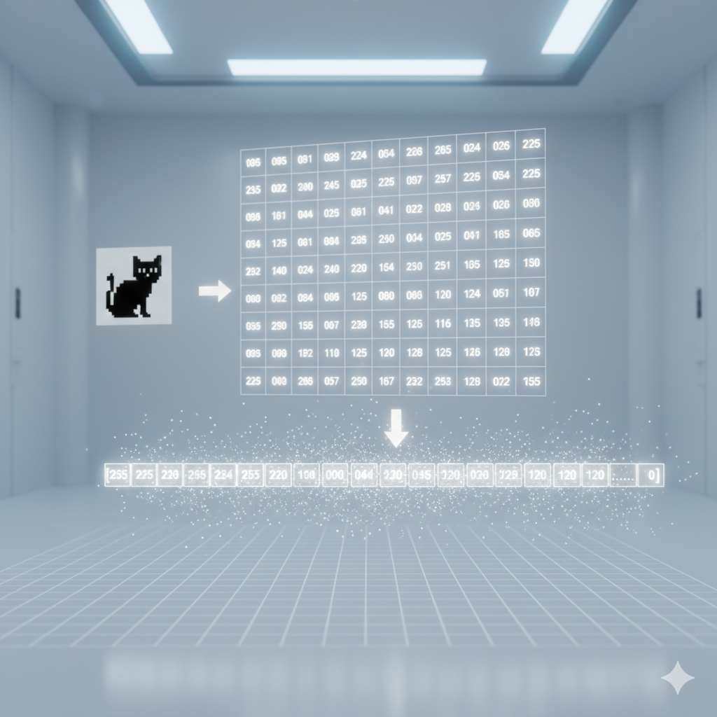
First, we need to see how images are represented in stable diffusion. Images are values from 0 (black) to 255 (white), usually organized as a tensor. A tensor has three matrices, each with arrays. Colored images use three matrices, black-and-white use one. For simplicity, let’s stick to black-and-white in a single matrix. (Stable diffusion actually takes a tensor.) This matrix flattens into a vector. For example, a 128×128 image becomes a vector of dimension 16,384. So, the model doesn’t hold tons of images but tons of vectors. Instead of images, we’re spreading vectors in pixel space. Now, recall we are drawing from this spread. Rather than full images, we’re drawing vectors. One might be [255,255,…,0], another [255,249,…,0]. This means we’re not just drawing the original images, but also ones slightly different from them.

Better Data Representations

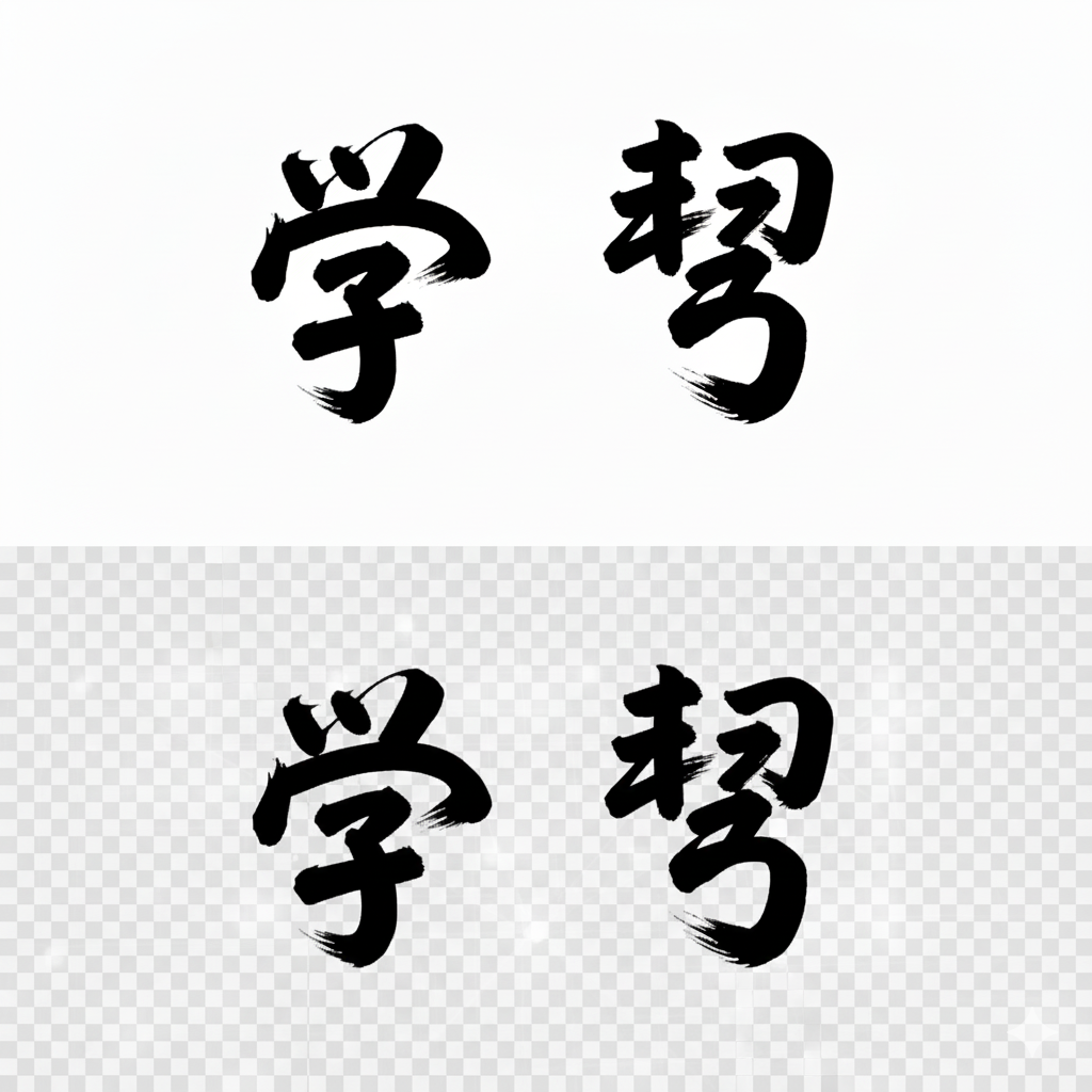
Most tasks don’t required machines to deal with full pixel-to-pixel vectors. For instance, if you want machines to differentiate these two Chinese Character images, then you might not even need to store the white background. Therefore, you can strip away some values from the vectors. This strip away action is called dimensionality reduction or more generally feature extraction. It is called dimensionality reduction because its reducing the amount of pivot in the vectors, and its called feature extraction because rather than keeping the raw data, it captures the essential features. In most machine learning tasks, most data are represented in that way. Even in nature, species perceives the external environment by only keeping keeping features.

VAE

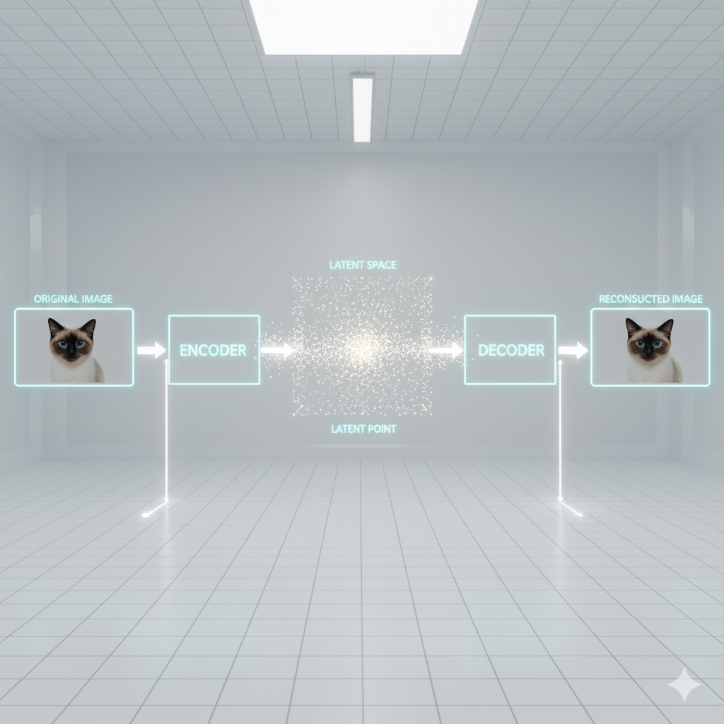
VAE (Variational Autoencoder) Components In stable diffusion, reduced vectors are called latent points. Together, they form the latent space. The VAE has three parts: encoder, latent space, decoder.

• The encoder compresses an image into a simpler vector.
• These vectors are stored in the latent space.
• The decoder reconstructs the image from the compressed vector.

In short, VAE removes non-essential features, then rebuilds the image from this simplified version.

Before VAE : AE

Before going further, we need to mention AE, the predecessor of VAE, and why VAE was born. The AE (autoencoder) also strips away non-essential features from raw data. But it had two weak points.

1. Discontinuity. AE does not ensure nearby points in latent space decode to similar outputs. A point near the code of a cat face might produce nonsense or even a distorted dog. Neighbors don’t guarantee smooth, meaningful transitions.
2. Incompleteness. AE does not fill the latent space with meaningful codes. Picking a random point often gives nothing sensible.

VAE fixes this by enforcing continuity and completeness. It makes similar latent points cluster together and keeps the space bounded.

Intuitively, think of latent space as a ball filled with points. In AE, the ball has gaps and unrelated contents may sit close. In VAE, points are rearranged to leave no gaps and group similar content together.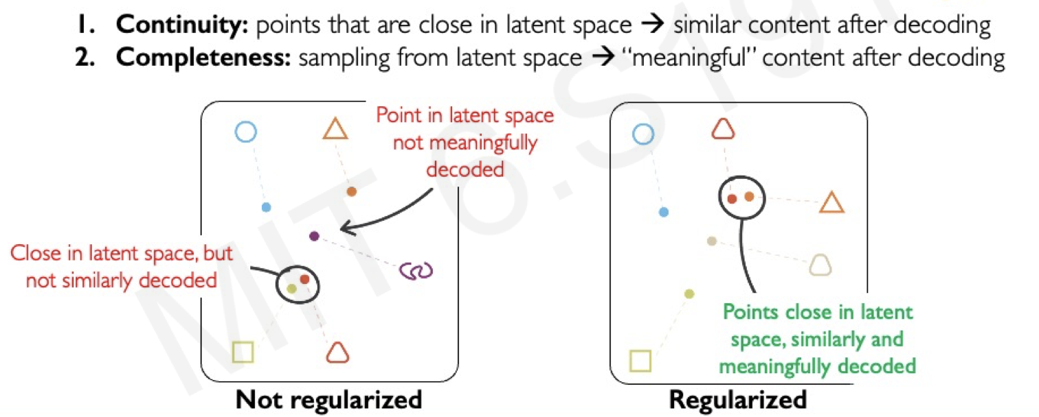

Loss of VAE

The loss function of AE is simply calculating the pixel-to-pixel difference to check the original image is similar to reconstructed image. This is formally expressed as the MSE between original image and the reconstructed image.

Previously, we point out that placing unalike contents nearby or placing a gap without contents in a latent space creates issues. Therefore, we need to rellocate so the latent is continuous and complete. To do this, on top of AE’s loss function, we add another term called kl divergence. This KL divergence regularization essentially helps rellocate those points, and organize the latent space more compact and complete.

Noise and Denoising Intuition

Earlier before, we explain the core mechanism diffusion, but rarely explain how they generate images. First, we dive into how model learns to generate images, then dive into how it generate images when a human prompts it.

Training

The training starts from a single image sample from the training set. The image is converted to a latent representation via VAE. Then, this latent image is placed into a latent space. To be precise, it takes the form of :

Now, the model starts corrupting the latent image into pure noise.
Intuitively, the image keeps its essential features (like kanji strokes without background), but becomes a gray cloud with random speckles.
This corruption is not one step, but many small steps, each adding a bit of noise until the latent is fully noise.
This multi-step noise addition is called the forward process.

Starting from the pure noised latent image, we aim to reconstruct the original.
Since the model can’t do this directly, a neural network learns to predict the noise that was added.
Once predicted, this noise is subtracted from the noisy latent to produce a cleaner latent.
This is one denoising step, repeated multiple times until we recover the clean latent image. This entire multi step is called the backward proces.

Formally, the model corrupts the latent image step by step with noise, giving

From the noisy latent, the model predicts the noise and subtracts it, giving

Note that, the forward process can differ by training images. In specific, each images are corrupted with different time points.

Training (Alternative Perspective)

You might wonder how these two processes play out in latent space.

Diffusion models learn a probability distribution over the training dataset, where each image is represented in a high-dimensional latent space. For visualization, we project this into lower dimensions (e.g., with UMAP), preserving only the essential structure.

In this landscape, peaks represent clean training images.
The forward process pushes a clean latent away from its peak, step by step, until it becomes pure noise.
The reverse process trains the network to walk back, starting from noise and removing it step by step to recover the clean image.

Together, this forms a single training iteration.
But in practice, we want the network to learn many noisy paths, not just one, so it becomes robust to different corruption trajectories.

For example, a red panda image might have its ears corrupted early in one path and later in another.
Even if the network sees only the nose at first, it still learns to walk back to the same clean red panda.
In short, the network generalizes across many noise patterns.

This is why diffusion models require many epochs—each training step only teaches the model to generalize from a single noisy image.

Inference

Now, once the neural network has learned how to denoise different latent images with different trajectories, it is now ready to generate images. In fact, capability of doing this are all stored in the backward process weights.

The process of generating an image, taking/sampling a point in the latent landscape space, and denoise back to a desired clean image with those stored weights.

Note that, we can also choose to generate image that never existed in the training images. This is because the model has not only learn the exact pixel-to-pixel training images, but also learn the variation of it such as a clean red panda but its nose is altered.

Furthermore, you may also choose interpolate an image by creating a smooth transition between two images. For instance, in the latent space, an image of a red panda face will be close to an image of a racoon face as they look alike. So, if your model end up denosing towards between those images, you will likely get an animal face that’s red panda like but also racoon like.

This is an example of a kind of interpolate that’s pairwise interpolation. In addition, you may choose bilinear interpolation where you pick 4 images as your anchors, and generate a new image between all of those.

Conditioning

Intuition

Till now, we have only focused purely on how the diffusion part works, but on top of that there is conditioning.
Conditioning is what makes Stable Diffusion able to process a text prompt and generate an image aligned with it.

In essence, conditioning narrows down the latent space. By restricting the space, the model samples only from regions consistent with the prompt, making generation more targeted.
To illustrate, without conditioning the model would sample from the entire latent space, producing some generic image.
With conditioning, if the prompt is “elephant”, the model samples from a scoped region of the latent space, and the generated image reflects the features of an elephant.

Intuition (Distribution)

In distribution terms, conditioning in latent space is like a joint distribution, which describes the probability of two events happening together.

For example, let

The joint distribution is written as

the probability of your mom getting strawberry cake given that she already picked coffee.

From this, we can condition:

Using this example, we can relate back to images.
Without conditioning, the model samples from the full distribution

producing a generic image.
With conditioning, the model samples from the conditional distribution

where (y) is the text prompt (e.g., “elephant”).
This restriction of latent space guides the model to generate an elephant image consistent with the prompt.

Unet

We have discussed how Stable Diffusion generates images aligned with text. Before diving further, we need to see how denoising works — specifically, how corrupted latent images are reconstructed. This task is done by the U-Net.

The process is as follows: the U-Net takes a corrupted latent image and passes it through its highest layer. On the encoder side, it extracts global features such as the overall Kanji composition, then passes them to the decoder side to predict and remove noise. This repeats at lower layers: deeper layers capture local features like edges and shapes, which are then used to refine the reconstruction.

Self Attention

So far we described a regular U-Net, but Stable Diffusion adds an extra component that boosts reconstruction quality: self-attention and cross-attention.

Self-attention is the key to why these models can generate sophisticated images, like placing text on a school whiteboard. Its purpose is to capture long-range dependencies. Unlike convolution, where each feature only sees its neighbors, self-attention lets any part of the image communicate directly with any other part.

Here’s how it works. For each latent image, a patch (Q) queries all other patches. Each patch (K) presents what it represents—for example, a furry edge of a cat. Q and K are dot-multiplied to produce an attention score, which measures how relevant each patch is to the query. Finally, these scores weight the values (V), the actual feature content, producing a context-dependent representation of the patch.

Cross Attention

The purpose of cross attention is to guide the denoising process so it aligns with the text prompt. In contrast to self attention, the query stays as image patches, but the keys and values come from the text prompt. Intuitively, certain phrases from the prompt are focused, so a specific region or shape is emphasized in the image patch.

For instance, take the prompt “a white horse in the park”. In the cross attention maps, the phrase “horse” strongly reflects the horse shape in the image, while the phrase “park” strongly reflects the background. These cross attention layers are added into some intermediate layers of the U-Net. Before the latent image from the decoder is passed to the encoder, it infuses or concatenates this cross attention map into the latent image. By doing this, the U-Net reconstructs the original image in alignment with the text.

Wrap Up

This process of taking one latent image and passing it through all layers of the decoder and encoder of the U-Net is a single step in the entire backward process. The model must repeat this step many times to fully reconstruct the latent image until it becomes clean. Once it fully reconstruct the latent image, the VAE encoder takes that reconstructs back to the original pixel to pixel image. And, that’s how you get an image generated that a naked eye can view.